Metabolic crosstalk on the Slide-TCR-seq human lung RCC dataset

In this tutorial, we demonstrate how we can use Harreman to perform metabolic crosstalk both at the cell-type-agnostic and cell-type-specific levels. For this, we will build on the metabolic zonation tutorial to infer metabolite exchange events that are specific to the previously defined zones.

If you are unfamiliar with how Harreman can be used to delineate metabolic zones in the tissue, we recommend starting with the metabolic zonation tutorial. However, most of the functions that we will cover in this tutorial do not depend on the outputs generated in the previous tutorial. Therefore, if you are not interested in dividing the tissue into metabolic zones, the previous tutorial can be skipped. In this case, beware of the functions that make use of metabolic modules, as you won’t be able to successfully run them until the metabolic zonation results are stored in your AnnData.

Plan for this tutorial:

1. Loading the data.

2. Inferring cell-type-agnostic gene pair and metabolite crosstalk.

3. Computing interacting gene pair and metabolite scores.

4. Group spatially co-localized metabolites.

5. Correlation between metabolite group scores and metabolic module scores.

Loading the dataset

In this tutorial, we will work with the AnnData saved in the metabolic zonation tutorial.

import harreman
import os
import tempfile
import numpy as np
import pandas as pd
import scanpy as sc
import anndata as ad
import seaborn as sns
import matplotlib.pyplot as plt
import matplotlib as mpl
import itertools
from scipy.stats import pearsonr, wilcoxon, mannwhitneyu, ranksums, zscore
import random
from sklearn import linear_model
from scipy.stats import hypergeom, zscore
import scipy.stats as stats
from statsmodels.stats.multitest import multipletests
from plotnine import *
from matplotlib.patches import Patch
from scipy.cluster.hierarchy import fcluster
import math
from collections import Counter
import warnings
warnings.filterwarnings("ignore")

adata = harreman.read_h5ad('Slide_seq_lung_metabolic_zonation.h5ad')

Cell-type-agnostic metabolic crosstalk

Firstly, we extract the metabolite and ligand-receptor interaction information for cellular crosstalk inference using the extract_interaction_db function. For this, we need to specify the organism the dataset corresponds to (with the species parameter), indicate if we want to load only transporter information from HarremanDB (database='transporter'), only ligand-receptor information from CellChatDB (database='LR'), or both of them (database='both'). In case we don’t want to restrict the interactions to the extracellular space, we can use the extracellular_only parameter with the False value.

Here, we load both databases from human and we restrict the interactions to the extracellular space.

harreman.pp.extract_interaction_db(adata, species='human', database='both', verbose=True)

We then compute the neighborhood graph using the compute_knn_graph function. For this, we need to specify the latent (or observed) space we are using to compute our cell metric with the compute_neighbors_on_key parameter. Further, only one of compute_neighbors_on_key or distances_obsp_key is needed in order to run the function. Similarly, either the neighborhood_radius or the n_neighbors parameter needs to be used (the former needs to contain information in micrometers). The sample_key parameter is optional and is only required when more than one sample are present in the AnnData and we want to avoid having neighbors across different samples.

Here, we set weighted_graph=False to just use binary, 0-1 weights and neighborhood_radius=100 to create a local neighborhood with a radius of 100 micrometers. Larger neighborhood sizes can result in more robust detection of correlations and autocorrelations at a cost of missing more fine-grained, smaller-scale, spatial patterns. Further, set sample_key='sample' to make sure there are no shared neighbors between samples.

harreman.tl.compute_knn_graph(adata, 
                        compute_neighbors_on_key="spatial", 
                        neighborhood_radius=100,
                        weighted_graph=False,
                        sample_key='sample',
                        verbose=True
                        )

Once the neighborhood graph is computed, genes can be filtered out to restrict the interactions to the most informative ones using the apply_gene_filtering function. For this, several options have been implemented. In our case, we use local autocorrelation (autocorrelation_filt = True parameter) with the Bernoulli distribution to model our data.

harreman.tl.apply_gene_filtering(adata, layer_key='counts', model='bernoulli', autocorrelation_filt = True, verbose=True)

To compute gene pairs, the compute_gene_pairs function is used. For this, cell type information can be used to compute cell-type-specific pairs. Here, as we are inferring crosstalk in a cell-type-agnostic way, ct_specific = False will be specified.

harreman.tl.compute_gene_pairs(adata, ct_specific = False, verbose=True)

To infer metabolic crosstalk, the compute_cell_communication function is used. To assess statistical significance, we can either use the parametric test (test = "parametric"), the non-parametric one (test = "non-parametric"), or both of them (test = "both"). If the parametric test needs to be computed, the model parameter needs to be specified, in addition to the raw counts layer (layer_key_p_test parameter). In this case, we use the Bernoulli distribution to model the count data. In case the non-parametric test is used, the number of permutations is specified through the M parameter (1000 by default), as well as the layer of the raw or normalized count data (layer_key_np_test parameter). In our case, we use the log-normalized counts to infer crosstalk and assess its significance through the non-parametric test.

harreman.tl.compute_cell_communication(adata, model='bernoulli', M = 1000, test = "both", layer_key_p_test='counts', layer_key_np_test='log_norm', verbose=True)

We then select statistically significant interactions (FDR < 0.05) from the non-parametric test (specified in the test parameter).

harreman.tl.select_significant_interactions(adata, test = "non-parametric", threshold = 0.05)

Computing gene pair and metabolite interacting scores

To visualize the interactions at the gene pair and metabolite levels in the tissue, the compute_interacting_cell_scores is used. The test parameter is analogous to the compute_cell_communication function, but, instead of using it to compute statistical significance (for this only the non-parametric test is used), we use it to specify if we want to compute the values using the raw counts (used for the parametric test) or the log-normalized counts (used for the non-parametric test). Here, we consider both of them, but we will eventually focus on the scores computed using the log-normalized counts. Additionally, as assessing the statistical significance using the non-parametric test can take a long time in this case, only the parametric one is used. However, as the parametric test has not been presented in the manuscript for this particular statistic, we will not consider significance values and will select relevant spots for each metabolite using a different approach.

harreman.tl.compute_interacting_cell_scores(adata, test = "both", compute_significance='parametric', verbose=True)

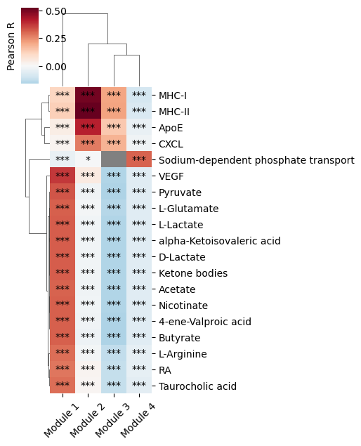
We then compute the correlation between the metabolite (or gene pair) scores and the metabolic module scores defined in the metabolic zonation tutorial. For this, the metabolite (or gene pair) scores computed in the non-parametric test (using the log-normalized counts) are considered. To specify whether we want to focus on gene pair or metabolite scores, the interaction_type parameter is used (with the metabolite or gene_pair value). Here, we run the function at the metabolite level.

harreman.tl.compute_interaction_module_correlation(adata, cor_method='pearson', interaction_type='metabolite', test='non-parametric')

Downstream analyses

We then visualize the correlation between metabolite scores and module scores.

harreman.pl.plot_interaction_module_correlation(adata, x_rotation = 45, figsize = (5,6), threshold = 0.25)

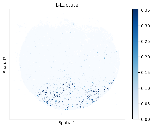
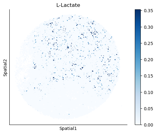
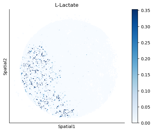
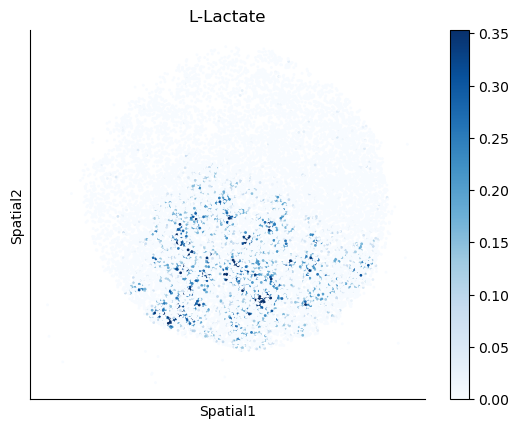
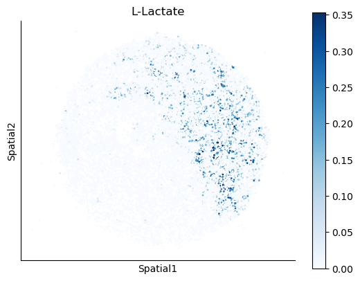
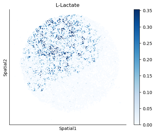
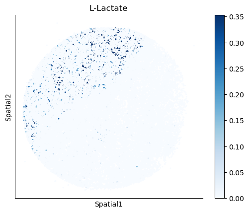
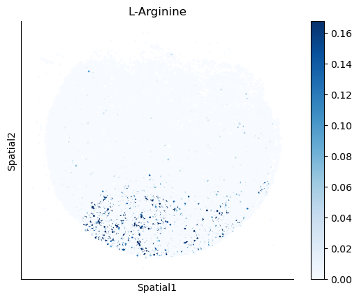
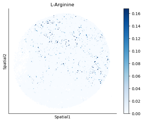
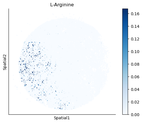
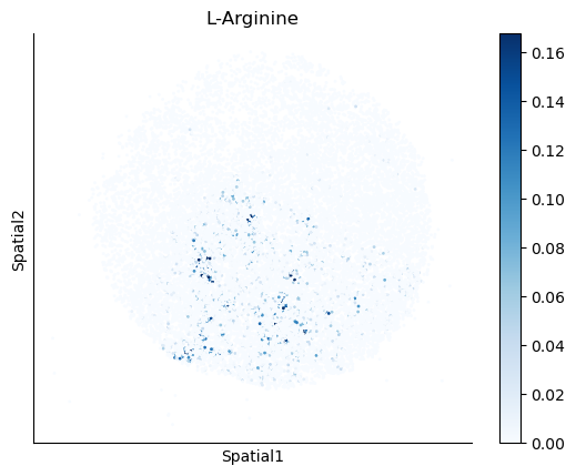
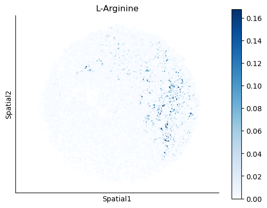
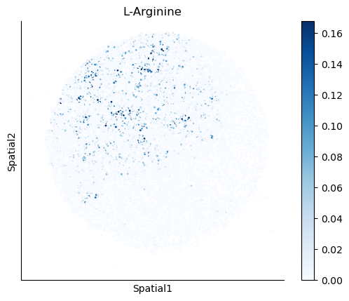
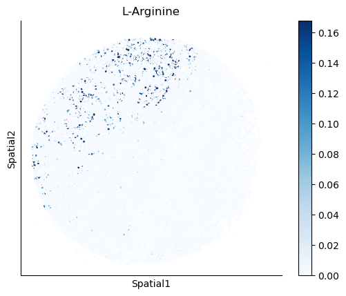
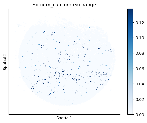
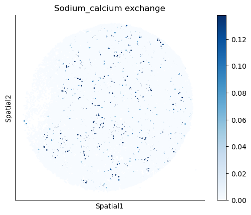
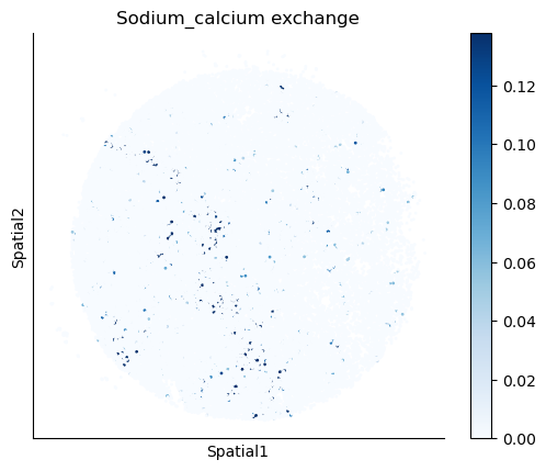
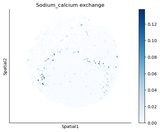
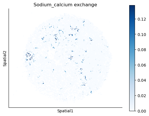
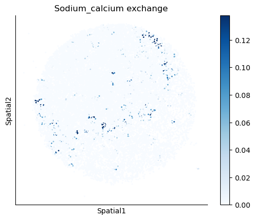
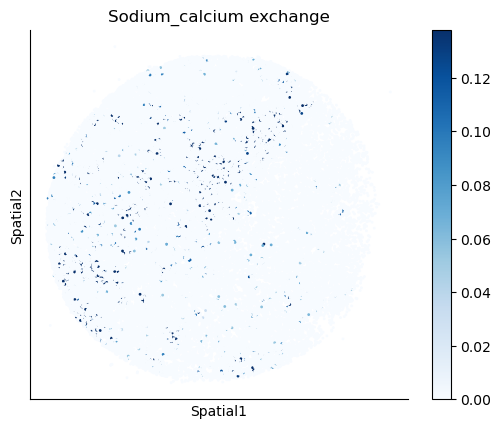
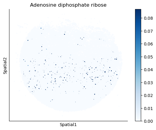
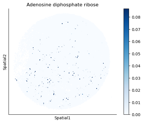
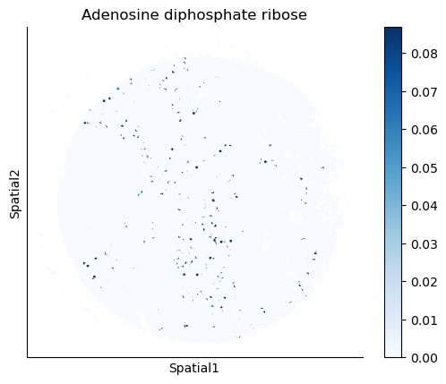
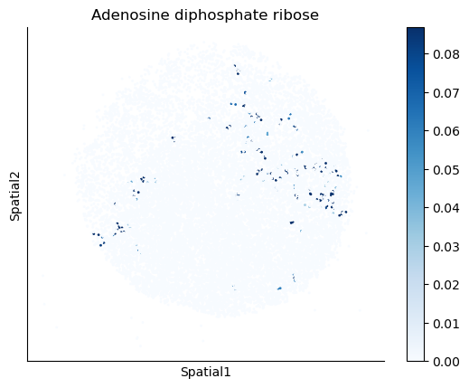
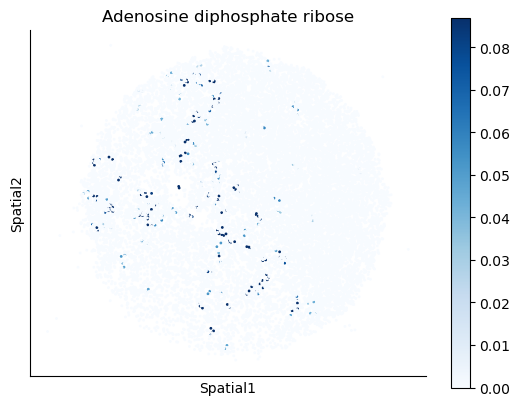
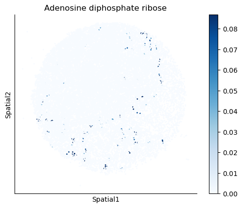
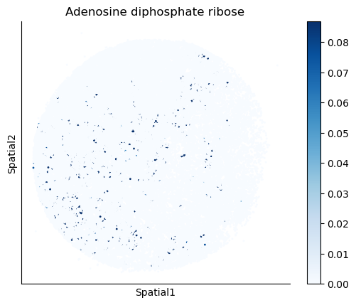
We select some metabolites to visualize them in the tissue.

metabolites = ['L-Lactate', 'L-Arginine', 'Sodium_calcium exchange', 'Adenosine diphosphate ribose']
harreman.pl.plot_interacting_cell_scores(adata, interactions=metabolites, test='non-parametric', coords_obsm_key='spatial', s=1, vmin='p1', vmax='p99', only_sig_values=False, normalize_values=True, cmap='Blues', sample_specific=True)

Puck_220408_20
Puck_220408_13
Puck_220408_15
Puck_200727_09
Puck_200727_10
Puck_200727_08
Puck_220408_14
Puck_220408_20
Puck_220408_13
Puck_220408_15
Puck_200727_09
Puck_200727_10
Puck_200727_08
Puck_220408_14
Puck_220408_20
Puck_220408_13
Puck_220408_15
Puck_200727_09
Puck_200727_10
Puck_200727_08
Puck_220408_14
Puck_220408_20
Puck_220408_13
Puck_220408_15
Puck_200727_09
Puck_200727_10
Puck_200727_08
Puck_220408_14

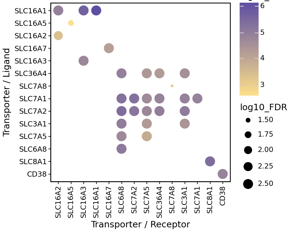
We can also identify which gene pairs belonging to the metabolites of interest have a significant spatial co-expression.

cell_communication_df = adata.uns['ccc_results']['cell_com_df_gp_sig'].copy()

gene_pairs_per_metabolite = adata.uns['gene_pairs_per_metabolite']
    
def to_tuple(x):
    # Recursively convert lists to tuples
    if isinstance(x, list):
        return tuple(to_tuple(i) for i in x)
    return x

metabolite_gene_pair_df = pd.DataFrame.from_dict(gene_pairs_per_metabolite, orient="index").reset_index()
metabolite_gene_pair_df = metabolite_gene_pair_df.rename(columns={"index": "metabolite"})
metabolite_gene_pair_df['gene_pair'] = metabolite_gene_pair_df['gene_pair'].apply(
    lambda arr: [(to_tuple(gp[0]), to_tuple(gp[1])) for gp in arr]
)
metabolite_gene_pair_df['gene_type'] = metabolite_gene_pair_df['gene_type'].apply(
    lambda arr: [(to_tuple(gt[0]), to_tuple(gt[1])) for gt in arr]
)
metabolite_gene_pair_df = pd.concat([
    metabolite_gene_pair_df['metabolite'],
    metabolite_gene_pair_df.explode('gene_pair')['gene_pair'],
    metabolite_gene_pair_df.explode('gene_type')['gene_type'],
], axis=1).reset_index(drop=True)

if 'LR_database' in adata.uns:
    LR_database = adata.uns['LR_database']
    df_merged = pd.merge(metabolite_gene_pair_df, LR_database, left_on='metabolite', right_on='interaction_name', how='left')
    LR_df = df_merged.dropna(subset=['pathway_name'])
    metabolite_gene_pair_df['metabolite'][metabolite_gene_pair_df.metabolite.isin(LR_df.metabolite)] = LR_df['pathway_name']

metabolite_gene_pair_df = metabolite_gene_pair_df.set_index('metabolite')

def is_present(row, gene_pairs):
    gene1, gene2 = row['Gene 1'], row['Gene 2']
    return any(
        (gene1 in pair and gene2 in pair) if isinstance(pair, tuple) else False
        for pair in gene_pairs
    )

gene_pairs = metabolite_gene_pair_df.loc[metabolites]['gene_pair'].tolist()
cell_communication_df_filt = cell_communication_df[cell_communication_df.apply(lambda row: is_present(row, gene_pairs), axis=1)]

gene_pairs_filt = list(zip(cell_communication_df_filt["Gene 1"], cell_communication_df_filt["Gene 2"]))

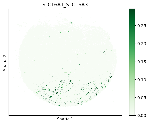
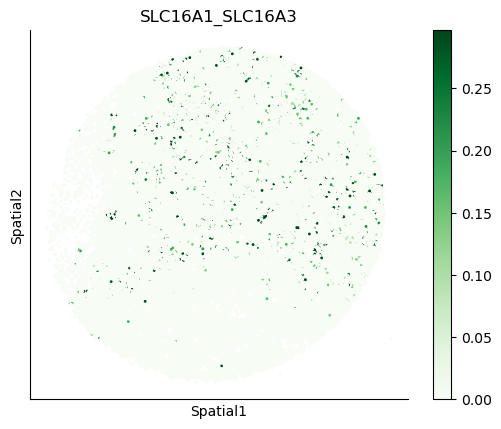
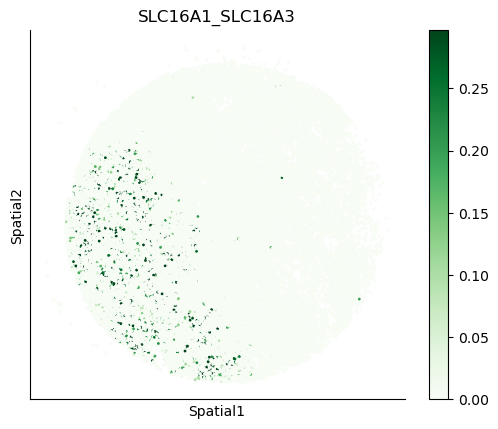
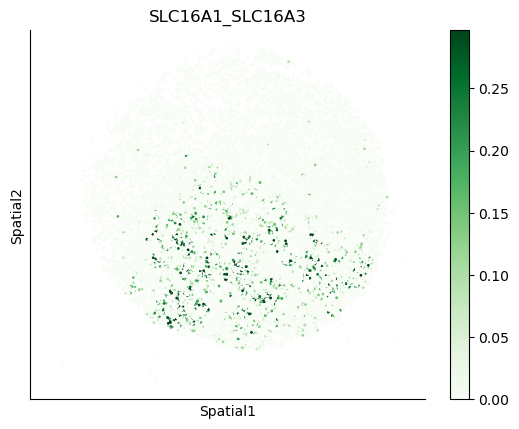
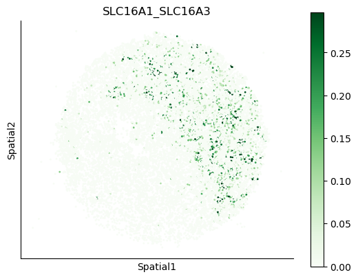
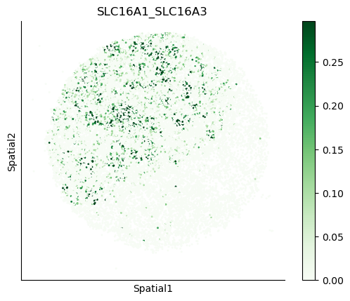
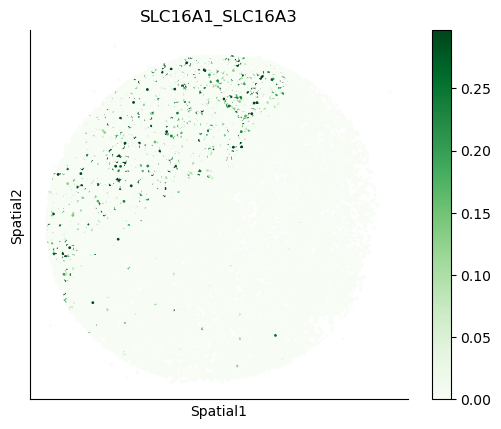
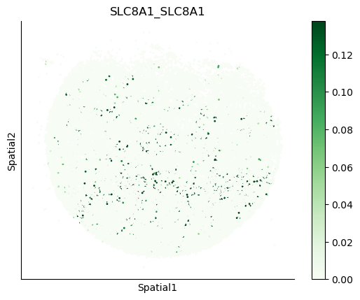
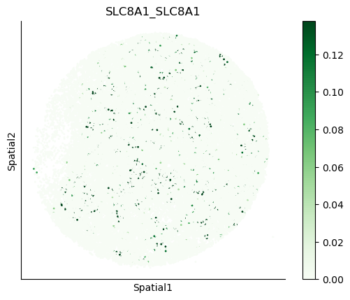
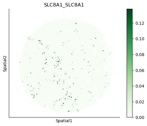
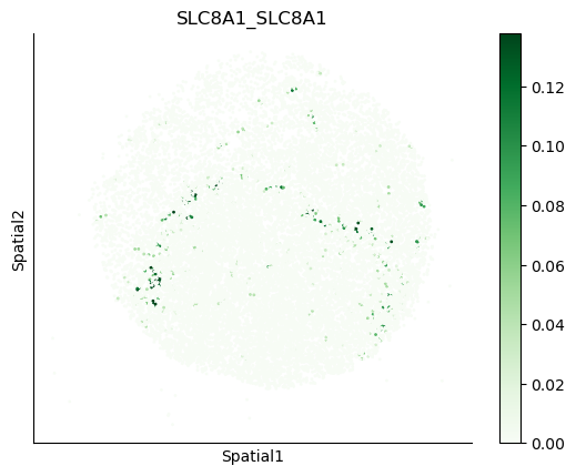
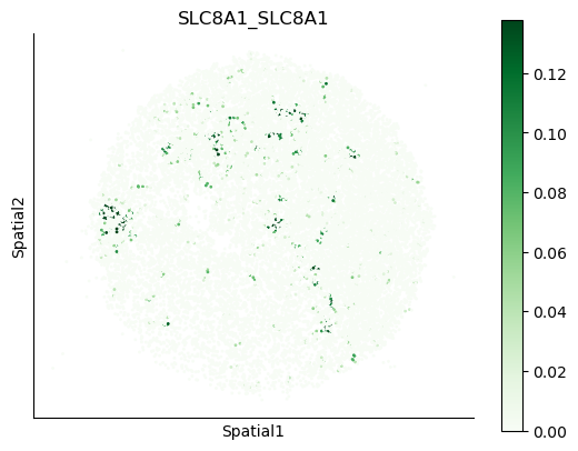
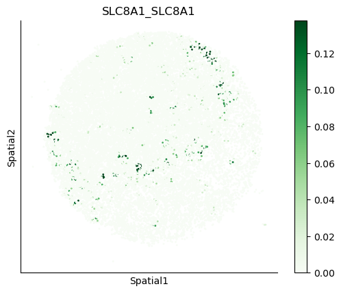
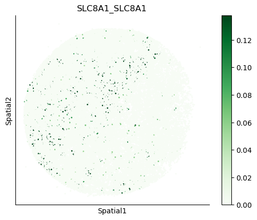
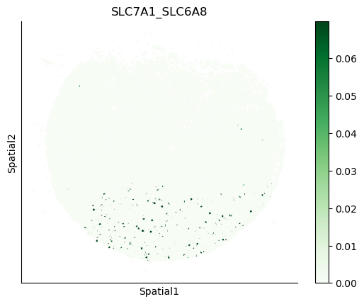
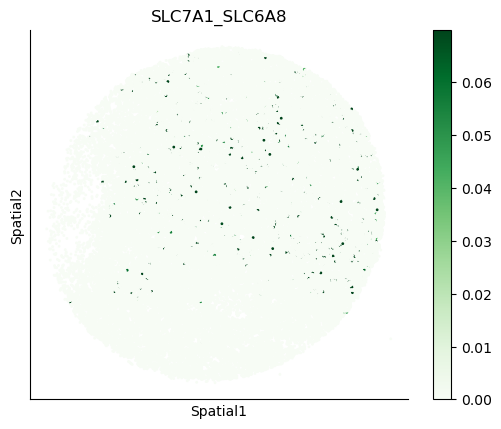
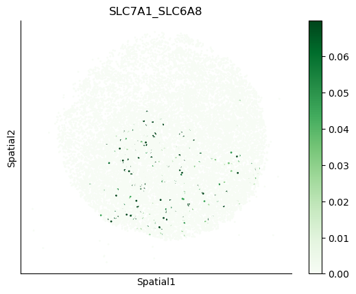
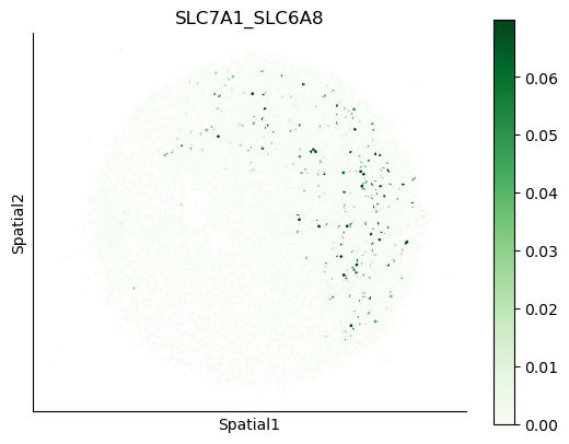
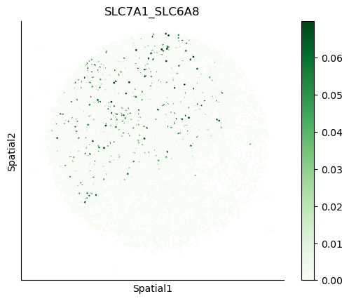
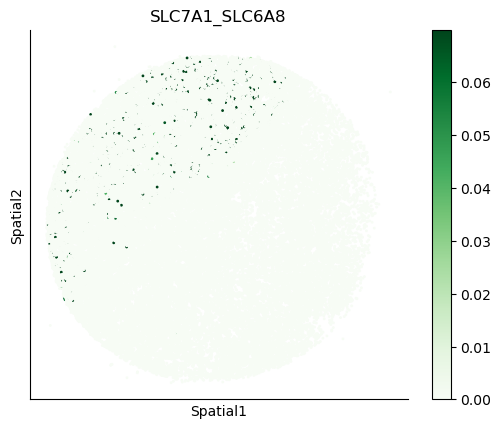
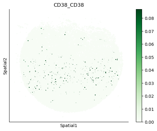
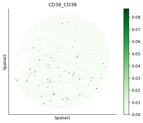
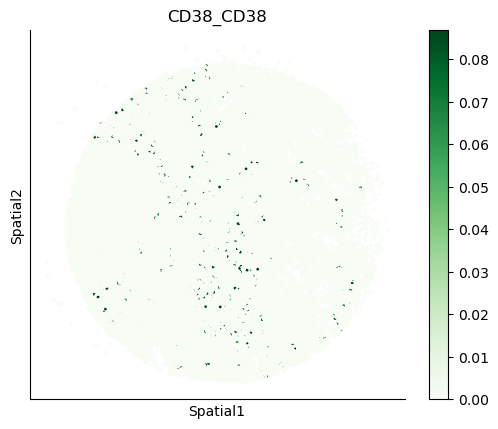
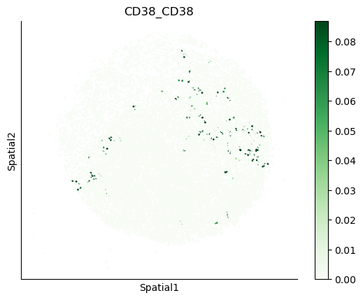
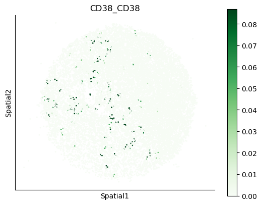
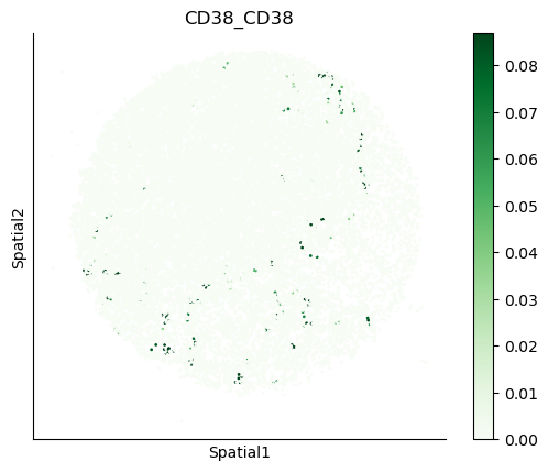
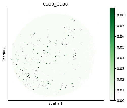
We can also visualize the spatial co-expression of some interesting transporter pairs.

gene_pairs_filt_plot = list(cell_communication_df_filt["Gene 1"] + '_' + cell_communication_df_filt["Gene 2"])

gene_pairs_filt_plot = ['SLC16A1_SLC16A3', 'SLC8A1_SLC8A1', 'SLC7A1_SLC6A8', 'CD38_CD38']

harreman.pl.plot_interacting_cell_scores(adata, interactions=gene_pairs_filt_plot, test='non-parametric', coords_obsm_key='spatial', s=1, vmin='p1', vmax='p99', only_sig_values=False, normalize_values=True, cmap='Greens', sample_specific=True)

Puck_220408_20
Puck_220408_13
Puck_220408_15
Puck_200727_09
Puck_200727_10
Puck_200727_08
Puck_220408_14
Puck_220408_20
Puck_220408_13
Puck_220408_15
Puck_200727_09
Puck_200727_10
Puck_200727_08
Puck_220408_14
Puck_220408_20
Puck_220408_13
Puck_220408_15
Puck_200727_09
Puck_200727_10
Puck_200727_08
Puck_220408_14
Puck_220408_20
Puck_220408_13
Puck_220408_15
Puck_200727_09
Puck_200727_10
Puck_200727_08
Puck_220408_14

gene_1 = ["_".join(pair[0]) if isinstance(pair[0], list) else pair[0] for pair in gene_pairs]
gene_2 = ["_".join(pair[1]) if isinstance(pair[1], list) else pair[1] for pair in gene_pairs]

def remove_duplicates(lst):
    seen = set()
    return [x for x in lst if not (x in seen or seen.add(x))]

gene_1 = remove_duplicates(gene_1)
gene_2 = remove_duplicates(gene_2)

cell_communication_df_filt['log10_FDR'] = -np.log10(cell_communication_df_filt['FDR_np'])
cell_communication_df_filt['log10_C'] = np.log10(cell_communication_df_filt['C_np'])

def convert_list_to_string(value):
    return '_'.join(value) if isinstance(value, list) else value

# Apply conversion to both columns
cell_communication_df_filt['Gene 1'] = cell_communication_df_filt['Gene 1'].apply(convert_list_to_string)
cell_communication_df_filt['Gene 2'] = cell_communication_df_filt['Gene 2'].apply(convert_list_to_string)

gene_1 = [gene for gene in gene_1 if gene in cell_communication_df_filt['Gene 1'].unique()]
gene_2 = [gene for gene in gene_2 if gene in cell_communication_df_filt['Gene 2'].unique()]

cell_communication_df_filt['Gene 1'] = cell_communication_df_filt['Gene 1'].astype('category')
cell_communication_df_filt['Gene 1'] = cell_communication_df_filt['Gene 1'].cat.reorder_categories(gene_1[::-1])

cell_communication_df_filt['Gene 2'] = cell_communication_df_filt['Gene 2'].astype('category')
cell_communication_df_filt['Gene 2'] = cell_communication_df_filt['Gene 2'].cat.reorder_categories(gene_2)

fig = (
ggplot(data=cell_communication_df_filt, mapping=aes(x='Gene 2', y='Gene 1', color='log10_C', size='log10_FDR')) 
+ geom_point()
+ scale_color_gradient(low = "#FEE08B", high = "#5E4FA2")
+ theme_classic() 
+ theme(plot_title = element_text(hjust = 0.5,
                                margin={"t": 0, "b": 5, "l": 0, "r": 0},
                                size = 14,
                                face='bold'),
        # legend_position = "none",
        axis_title_x = element_text(size = 11),
        axis_title_y = element_text(size = 11),
        axis_text_x = element_text(margin={"t": 0, "b": 0, "l": 0, "r": 10}, size = 9, colour='black', rotation=90),
        axis_text_y = element_text(margin={"t": 0, "b": 0, "l": 0, "r": 10}, size = 9, colour='black'),
        panel_border = element_rect(color='black'),
        panel_background = element_rect(colour = "black",
                                        linewidth = 1),
        figure_size=(5, 4)) + ylab('Transporter / Ligand') + xlab('Transporter / Receptor')
)
fig.show()

Group spatially co-localized metabolites

We now group spatially co-localized metabolites and assess if their presence is correlated with the predefined metabolic zones. For this, we will binarize the metabolite scores computed using the compute_interacting_cell_scores function, such that those spots with a value higher than 1 standard deviation above the mean will be assigned a value of 1, and 0 otherwise.

interacting_cell_scores_m = adata.uns['interacting_cell_results']['np']['m']['cs'].copy()
n=1
means = np.nanmean(interacting_cell_scores_m, axis=0)
stds = np.nanstd(interacting_cell_scores_m, axis=0)
thresholds = means + n*stds
interacting_cell_scores_m[interacting_cell_scores_m < thresholds] = 0

interacting_cell_scores_m = pd.DataFrame(interacting_cell_scores_m, index=adata.obs_names, columns=adata.uns['metabolites'])

interacting_cell_scores_m[interacting_cell_scores_m != 0] = 1

We create a new AnnData with the binarized metabolite scores to run the metabolic zonation pipeline.

metab_scores_adata = ad.AnnData(interacting_cell_scores_m)
metab_scores_adata.obs_names = adata.obs_names
metab_scores_adata.var_names = adata.uns['metabolites']

metab_scores_adata.obs['sample'] = adata.obs['sample']
metab_scores_adata.obsm['spatial'] = adata.obsm['spatial']

Here we compute the spatial proximity graph using the same parameters as before.

harreman.tl.compute_knn_graph(metab_scores_adata, 
                           compute_neighbors_on_key="spatial", 
                           neighborhood_radius=100,
                           weighted_graph=False,
                           sample_key='sample')

The code below is only run to filter out metabolites with all-zero values in at least one of the samples for subsequent pairwise correlation. We don’t select autocorrelated metabolites through this approach as they have already been selected using the select_significant_interactions function.

Here, the Bernoulli will be used, as the metabolite scores have been binarized and this is the best distribution to model the data.

harreman.hs.compute_local_autocorrelation(metab_scores_adata, model='bernoulli')

gene_autocorrelation_results = metab_scores_adata.uns['gene_autocorrelation_results']
metabolites = gene_autocorrelation_results.index

Pairwise correlation between binarized metabolite scores is also evaluated.

harreman.hs.compute_local_correlation(metab_scores_adata, genes=metabolites)

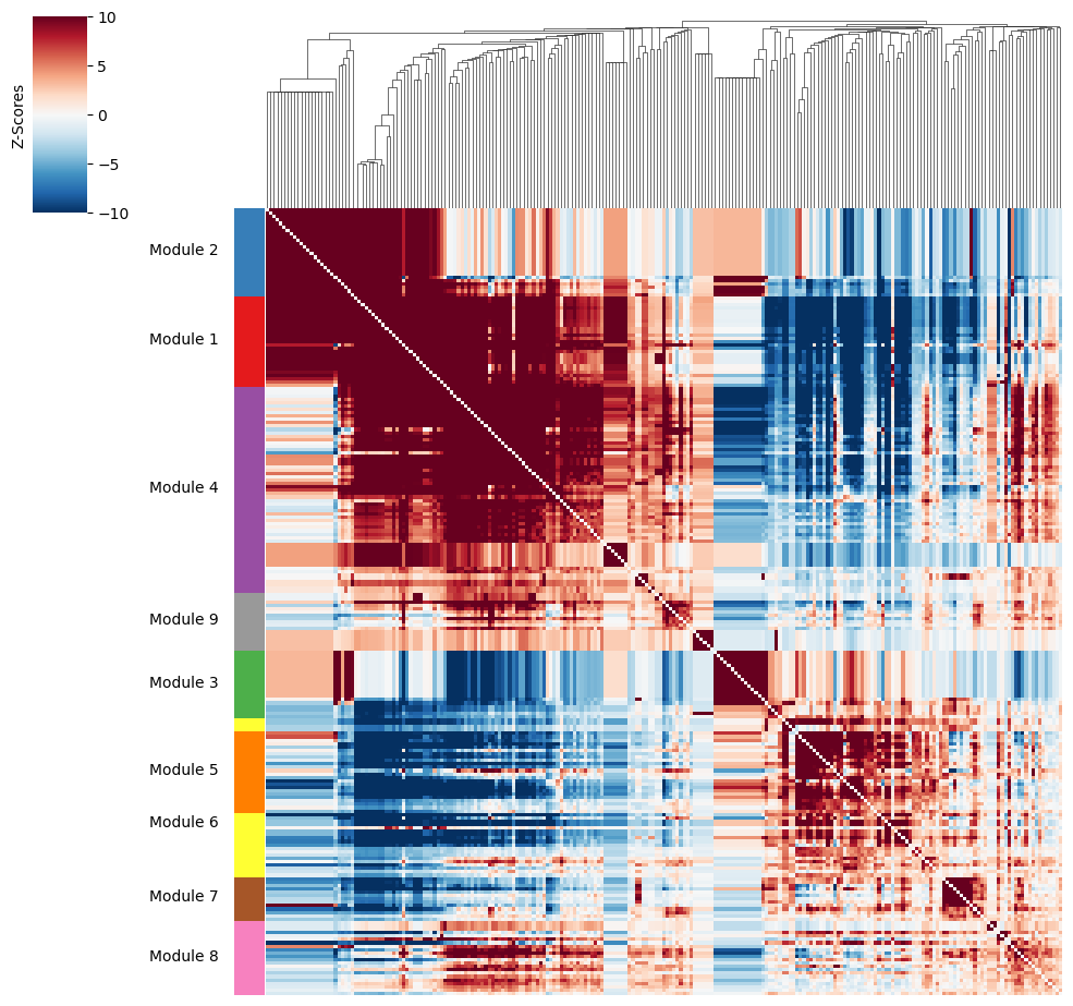
Then, metabolite groups are created.

harreman.hs.create_modules(metab_scores_adata, min_gene_threshold=10)

harreman.pl.local_correlation_plot(metab_scores_adata, mod_cmap='Set1')

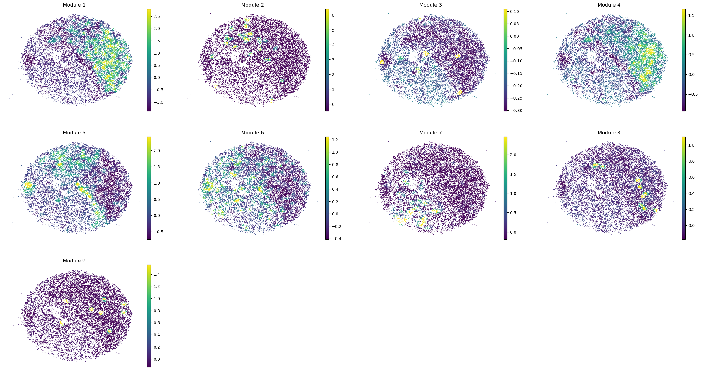
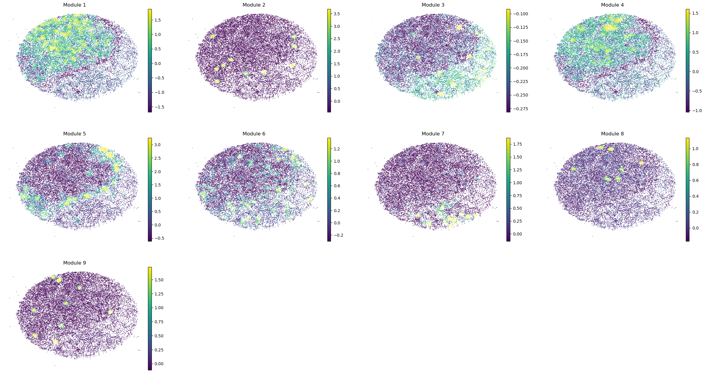
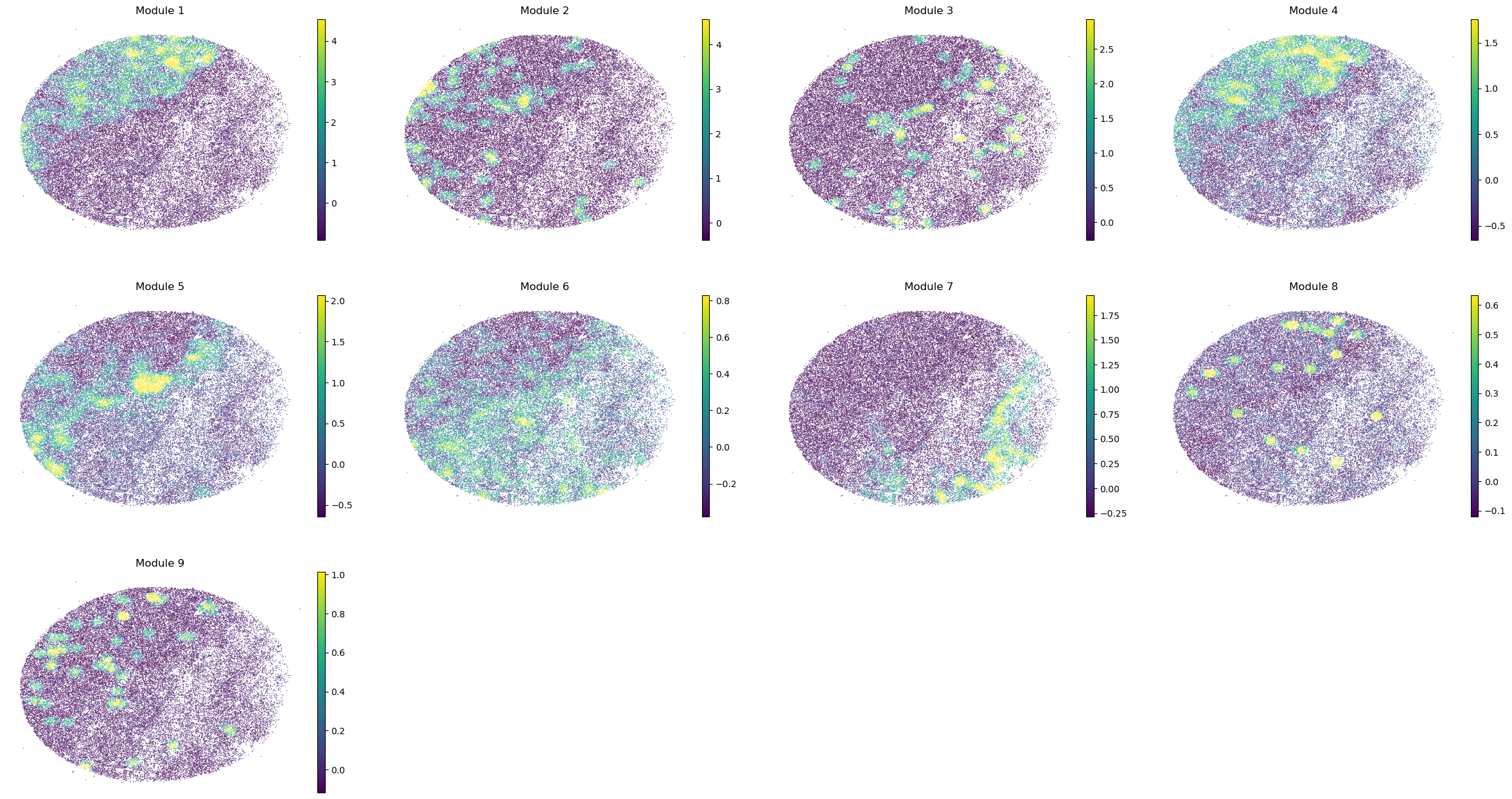
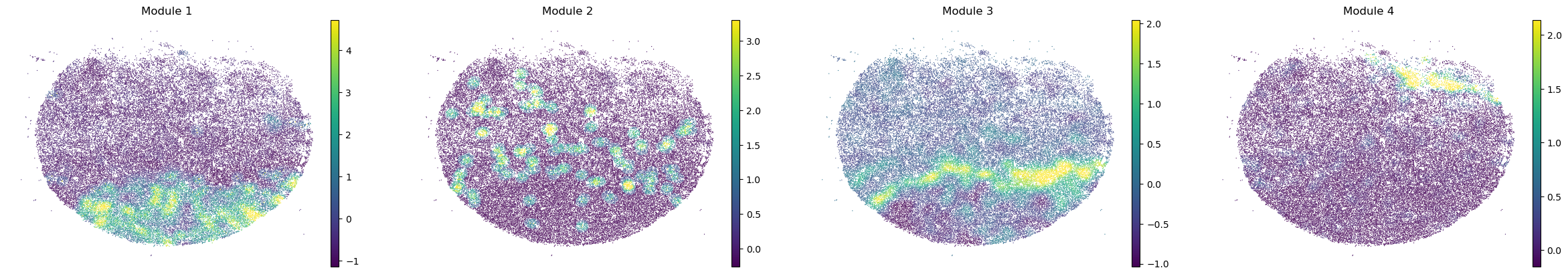
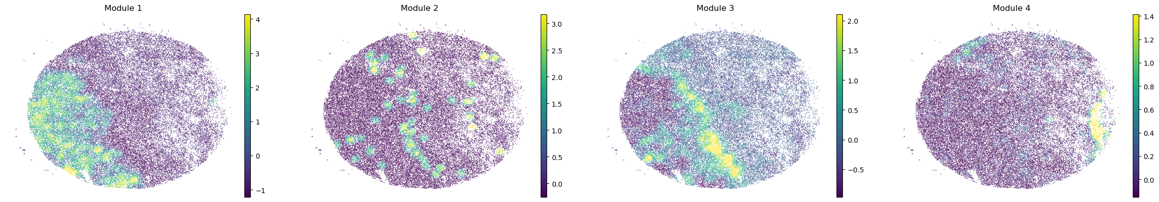
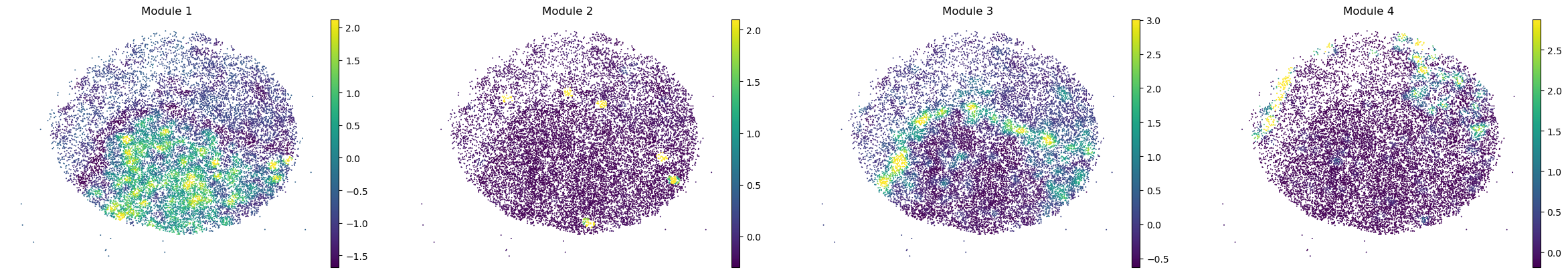
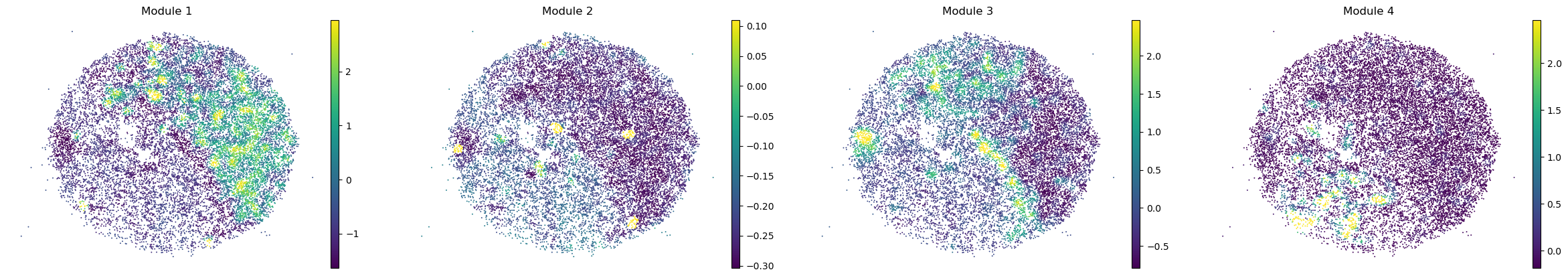
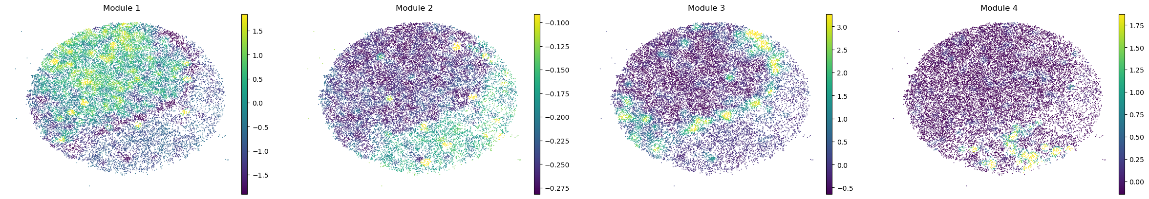
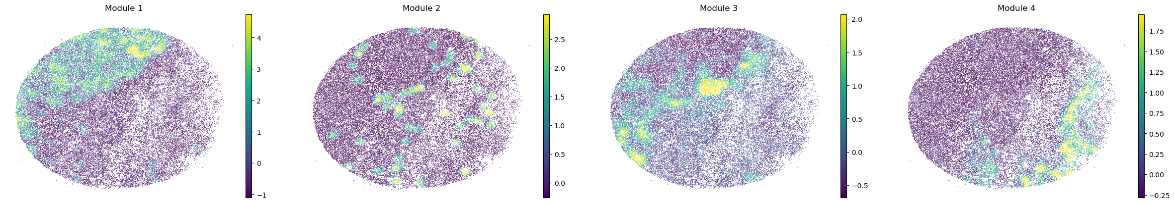
We also compute metabolite group scores to eventually correlate them with the previously computed metabolic module scores.

harreman.hs.calculate_module_scores(metab_scores_adata)

modules = metab_scores_adata.obsm['module_scores'].columns
metab_scores_adata.obs[modules] = metab_scores_adata.obsm['module_scores']

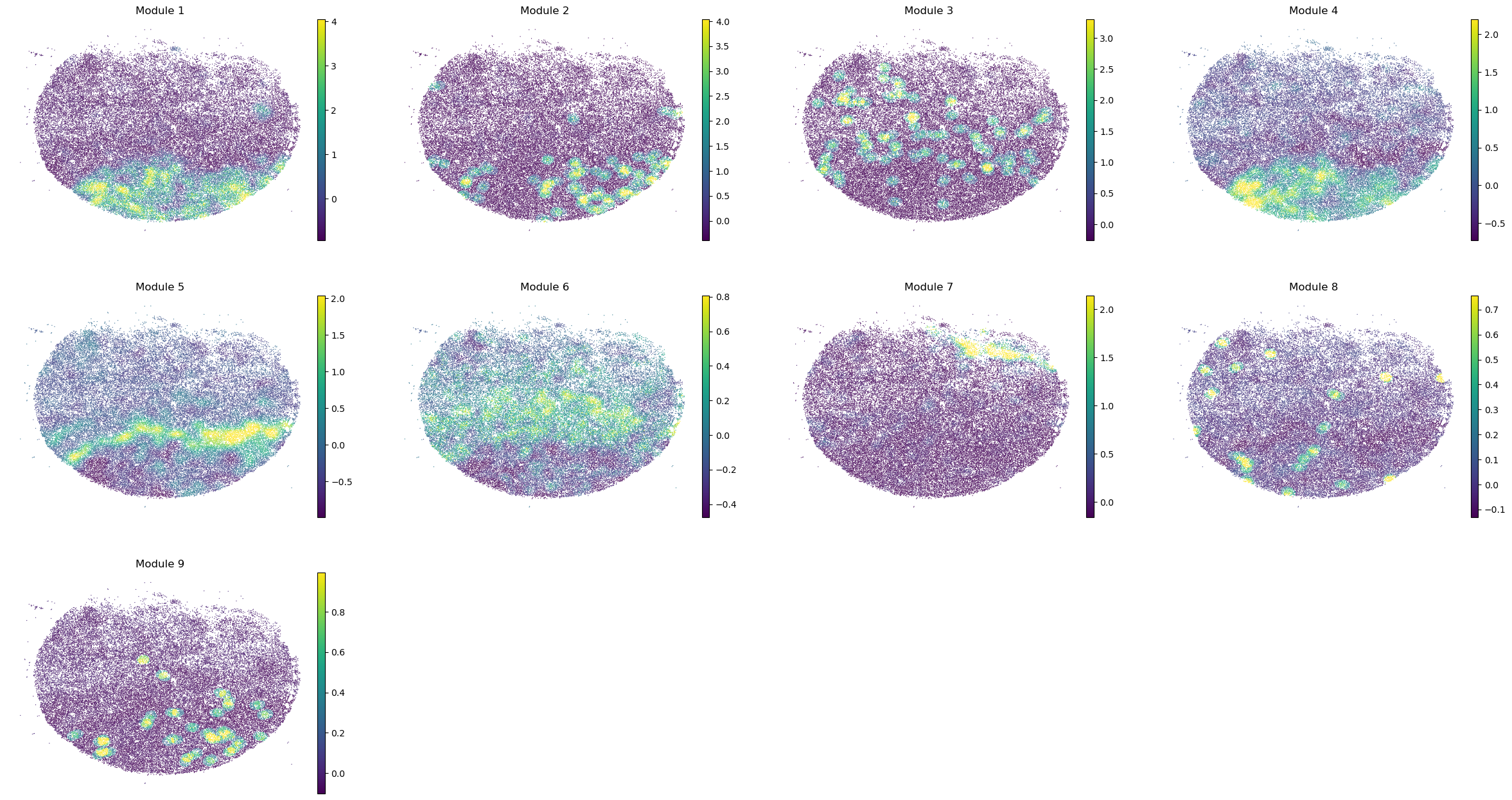
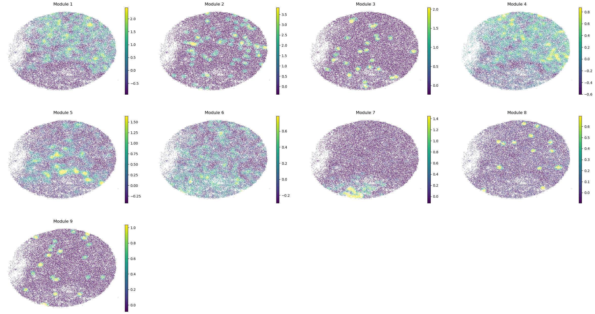
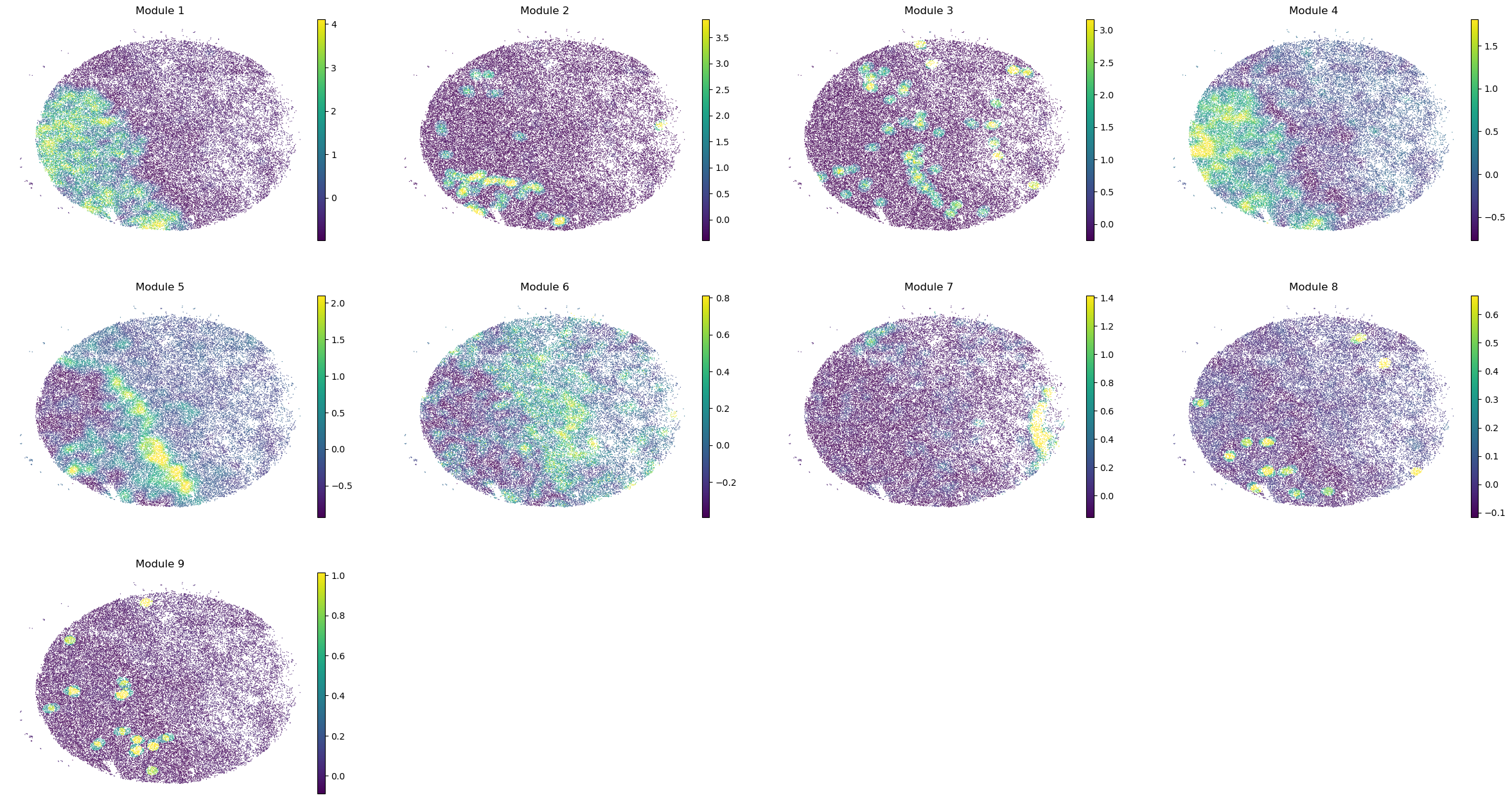
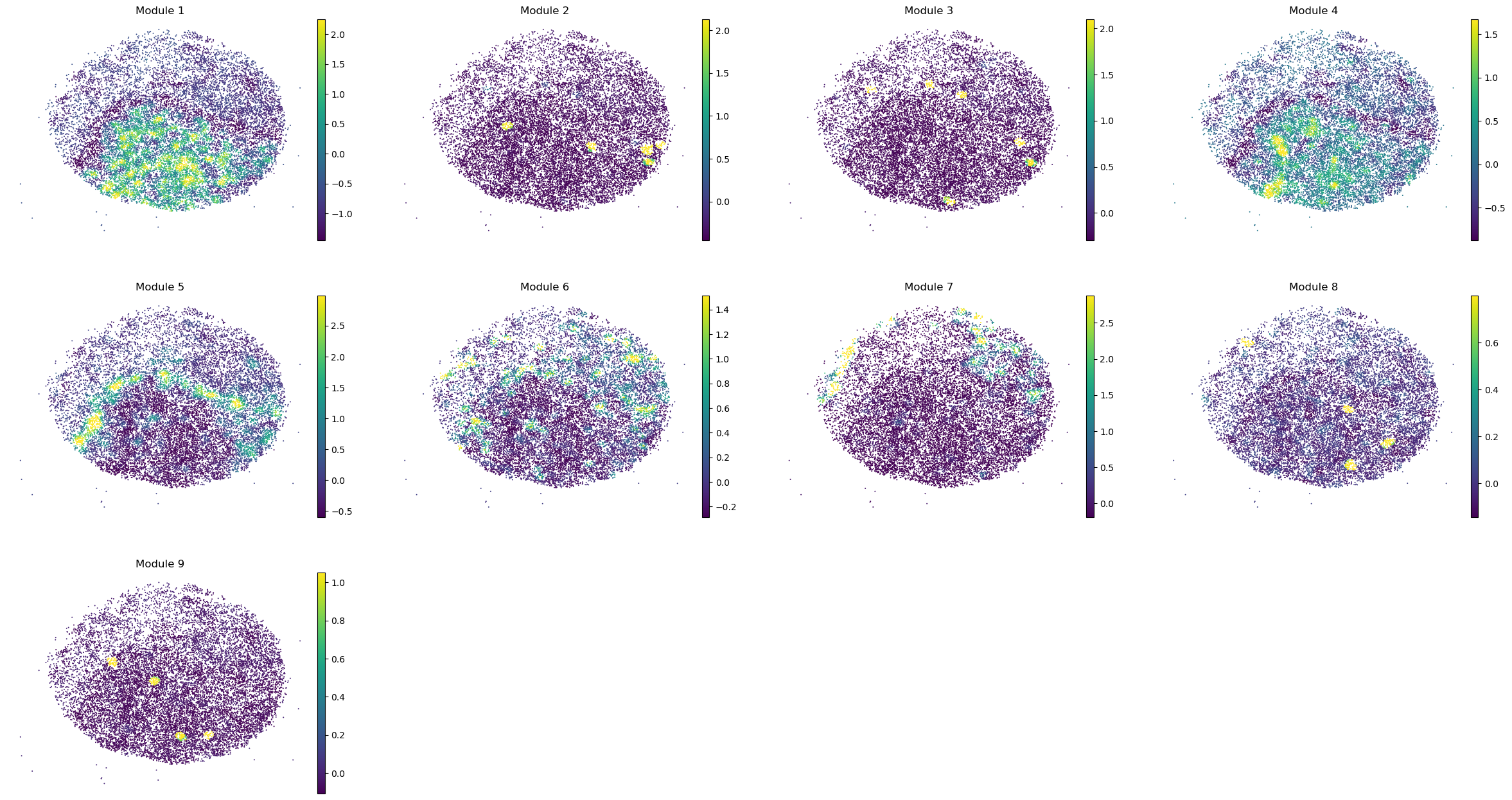
for sample in metab_scores_adata.obs['sample'].unique():
    print(sample)
    sample_adata = metab_scores_adata[metab_scores_adata.obs['sample'] == sample].copy()
    sc.pl.embedding(sample_adata, basis='spatial', color=modules, frameon=False, vmin="p1", vmax="p99", ncols=4)

Puck_220408_20
Puck_220408_13
Puck_220408_15
Puck_200727_09
Puck_200727_10
Puck_200727_08
Puck_220408_14

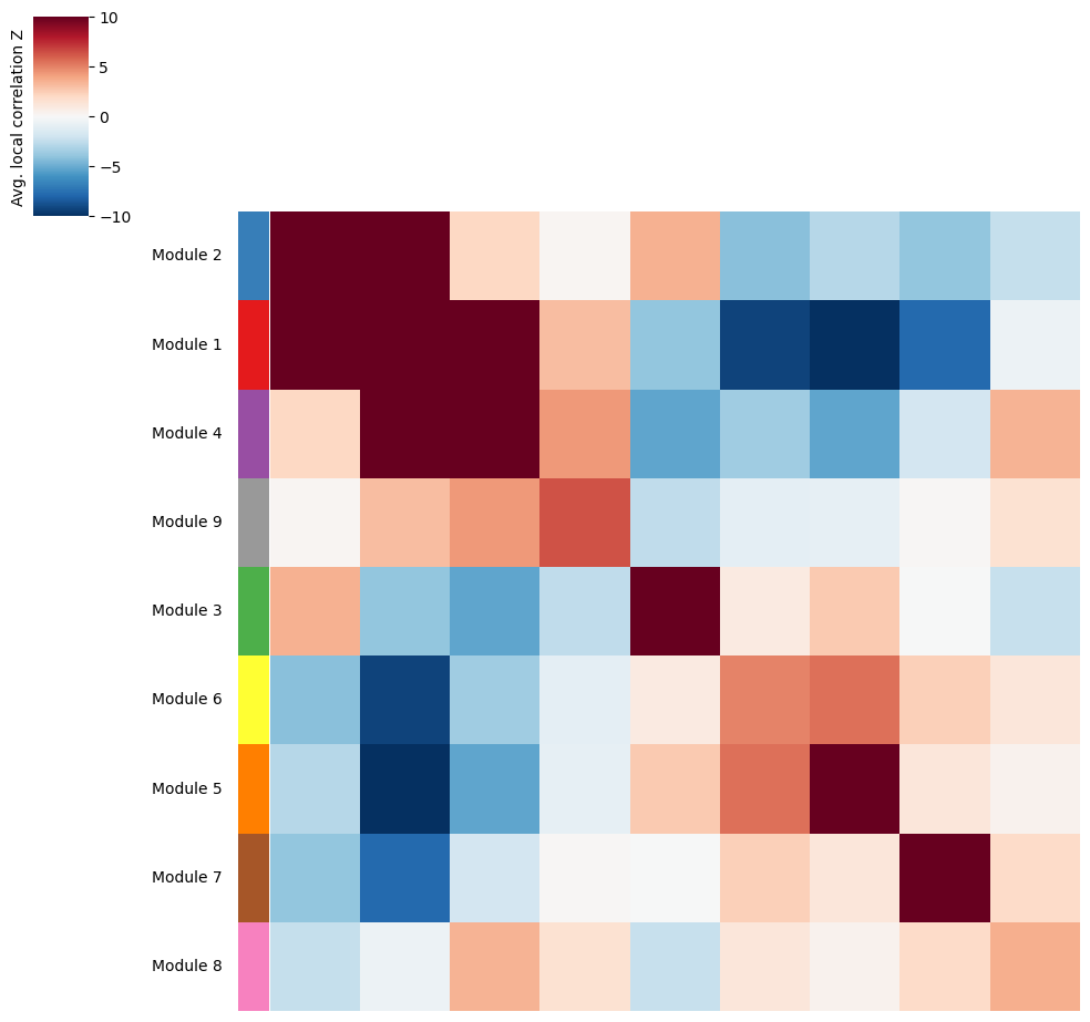
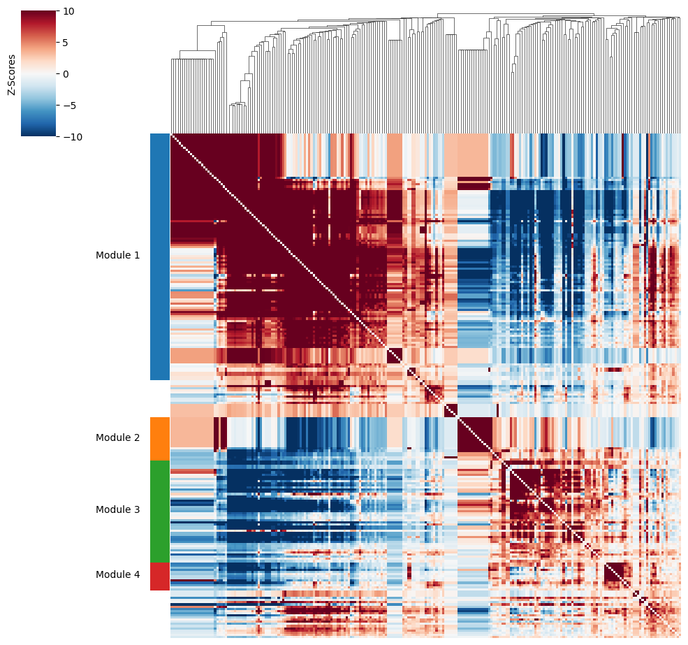
Once metabolite groups have been computed, we might want to group similar ones together or ignore unspecific or noisy groups. For this, we can visualize the average pairwise Z-scores between groups.

harreman.pl.average_local_correlation_plot(metab_scores_adata, col_cluster=False, row_cluster=False, mod_cmap='Set1', show=False)

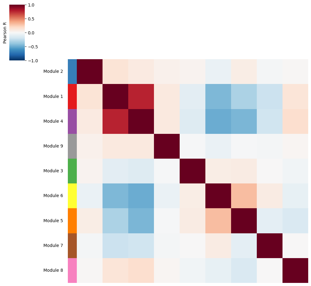
Additionally, we can also visualize the correlations between metabolite group scores to identify groups with a similar spatial pattern.

harreman.pl.module_score_correlation_plot(metab_scores_adata, col_cluster=False, row_cluster=False, mod_cmap='Set1', show=False)

Eventually, metabolite modules can also be grouped together into super-groups and we recompute the scores using the same approach as in the metabolic zonation pipeline.

super_module_dict = {
    -1: [8, 9],
    1: [1, 2, 4],
    2: [3],
    3: [5, 6],
    4: [7],
}

harreman.hs.calculate_super_module_scores(metab_scores_adata, super_module_dict=super_module_dict)

Finished computing super-module scores in 6.580 seconds

We can then visualize the pairwise correlation plot at the super-group level.

harreman.pl.local_correlation_plot(metab_scores_adata, use_super_modules=True, show=False)

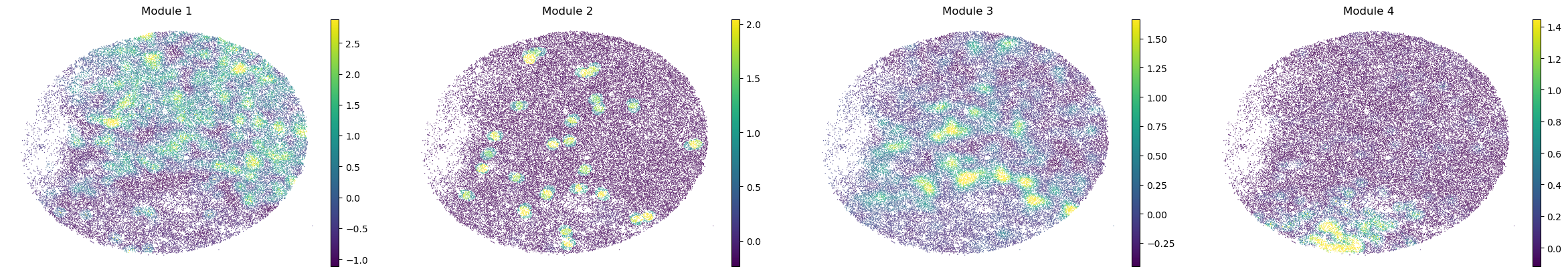
And super-group scores are computed.

super_modules = metab_scores_adata.obsm['super_module_scores'].columns
metab_scores_adata.obs[super_modules] = metab_scores_adata.obsm['super_module_scores']

for sample in metab_scores_adata.obs['sample'].unique():
    print(sample)
    sample_adata = metab_scores_adata[metab_scores_adata.obs['sample'] == sample].copy()
    sc.pl.embedding(sample_adata, basis='spatial', color=super_modules, frameon=False, vmin="p1", vmax="p99", ncols=4)

Puck_220408_20
Puck_220408_13
Puck_220408_15
Puck_200727_09
Puck_200727_10
Puck_200727_08
Puck_220408_14

Module / metabolite group correlation analysis

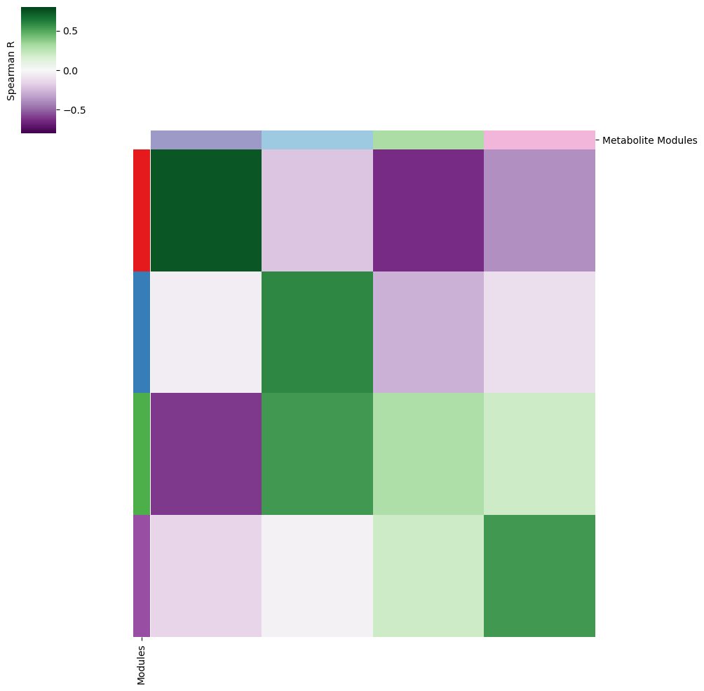
We compute the correlation between metabolic module scores and metabolite group scores.

common_cells = adata.obsm['module_scores'].index.intersection(metab_scores_adata.obsm['super_module_scores'].index)
df1a = adata.obsm['module_scores'].loc[common_cells]
df2a = metab_scores_adata.obsm['super_module_scores'].loc[common_cells]

corr = pd.DataFrame(index=df1a.columns, columns=df2a.columns, dtype=float)
for m1 in df1a.columns:
    for m2 in df2a.columns:
        corr.at[m1, m2] = df1a[m1].corr(df2a[m2], method='spearman')

colors = ["#E41A1C", "#377EB8", "#4DAF4A", "#984EA3", "#FF7F00", "#FFFF33", "#A65628", "#F781BF", "#999999"]
palette_m = {mod: colors[int(mod.split(' ')[1])-1] for mod in adata.obs['top_module'].dropna().unique()}

palette = {
    'Module -1': "#BDBDBD",
    'Module 1': "#9E9AC8",
    'Module 2': "#ABDDA4",
    'Module 3': "#9ECAE1",
    'Module 4': "#F1B6DA",
}

And we then can visualize the correlation results.

vmin=-0.8
vmax=0.8
cmap=sns.color_palette("PRGn", as_cmap=True)
yticklabels=False

row_colors1 = pd.Series(
    [palette_m[i] for i in corr.index],
    index=corr.index,
)

row_colors = pd.DataFrame({
    "Modules": row_colors1,
})

col_colors1 = pd.Series(
    [palette[i] for i in corr.columns],
    index=corr.columns,
)

col_colors = pd.DataFrame({
    "Metabolite Modules": col_colors1,
})

cm = sns.clustermap(
    corr,
    vmin=vmin,
    vmax=vmax,
    cmap=cmap,
    xticklabels=False,
    yticklabels=yticklabels,
    row_colors=row_colors,
    col_colors=col_colors,
    rasterized=True,
)

fig = plt.gcf()
plt.sca(cm.ax_heatmap)
plt.ylabel("")
plt.xlabel("")

cm.ax_row_dendrogram.remove()
cm.ax_col_dendrogram.remove()

plt.sca(cm.ax_row_colors)

# Find the colorbar 'child' and modify
min_delta = 1e99
min_aa = None
for aa in fig.get_children():
    try:
        bbox = aa.get_position()
        delta = (0-bbox.xmin)**2 + (1-bbox.ymax)**2
        if delta < min_delta:
            delta = min_delta
            min_aa = aa
    except AttributeError:
        pass

min_aa.set_ylabel('Spearman R')
min_aa.yaxis.set_label_position("left")

Cell-type-specific metabolic crosstalk

In the final step of the Harreman pipeline, we will perform cell-type-specific metabolic crosstalk inference by focusing on a few metabolites of interest and their corresponding significant gene pairs.

To assign cell types to spots, we can do different things. On the one hand, if the dataset contains single cells instead of spots (not in this case), we could directly annotate the cells and then run the pipeline directly. On the other hand, we could run DestVI (Lopez et al., Nature biotechnology, 2022) or another cell type deconvolution algorithm (such as cell2location; Kleshchevnikov et al., Nature biotechnology, 2022) to infer the cell type proportions in every spot and then either (1) assign the cell type with the highest (z-normalized) proportion to every spot, or (2) use the imputed cell-type-specific gene expression counts to achieve a higher resolution (cell types per spot).

Here, we will use the DestVI deconvolution results but, instead of running the algorithm on the imputed cell-type-specific counts, we will assign a given cell type (the one with the highest z-normalized proportion) to every spot.

temp_dir_obj = tempfile.TemporaryDirectory()

st_adata_path = os.path.join(temp_dir_obj.name, "Liu_et_al_human_lung_DestVI_v2.h5ad")
st_adata = sc.read(st_adata_path, backup_url='https://figshare.com/ndownloader/files/60231869')

adata = adata[adata.obs_names.isin(st_adata.obs_names)].copy()

cell_types = [ct for ct in st_adata.obsm['proportions'].columns if 'additional' not in ct]
df_z = st_adata.obsm['proportions'][cell_types].apply(zscore, axis=0)
assigned_cell_types = df_z.idxmax(axis=1)
adata.obs['cell_type'] = assigned_cell_types

We load the cell-type-agnostic crosstalk results to select the statistically significant gene pairs of the metabolites of interest.

metabolites = ['L-Lactate', 'L-Arginine', 'Sodium_calcium exchange', 'Adenosine diphosphate ribose']

cell_communication_df = adata.uns['ccc_results']['cell_com_df_gp_sig'].copy()

gene_pairs_per_metabolite = adata.uns['gene_pairs_per_metabolite']
    
def to_tuple(x):
    # Recursively convert lists to tuples
    if isinstance(x, list):
        return tuple(to_tuple(i) for i in x)
    return x

metabolite_gene_pair_df = pd.DataFrame.from_dict(gene_pairs_per_metabolite, orient="index").reset_index()
metabolite_gene_pair_df = metabolite_gene_pair_df.rename(columns={"index": "metabolite"})
metabolite_gene_pair_df['gene_pair'] = metabolite_gene_pair_df['gene_pair'].apply(
    lambda arr: [(to_tuple(gp[0]), to_tuple(gp[1])) for gp in arr]
)
metabolite_gene_pair_df['gene_type'] = metabolite_gene_pair_df['gene_type'].apply(
    lambda arr: [(to_tuple(gt[0]), to_tuple(gt[1])) for gt in arr]
)
metabolite_gene_pair_df = pd.concat([
    metabolite_gene_pair_df['metabolite'],
    metabolite_gene_pair_df.explode('gene_pair')['gene_pair'],
    metabolite_gene_pair_df.explode('gene_type')['gene_type'],
], axis=1).reset_index(drop=True)

if 'LR_database' in adata.uns:
    LR_database = adata.uns['LR_database']
    df_merged = pd.merge(metabolite_gene_pair_df, LR_database, left_on='metabolite', right_on='interaction_name', how='left')
    LR_df = df_merged.dropna(subset=['pathway_name'])
    metabolite_gene_pair_df['metabolite'][metabolite_gene_pair_df.metabolite.isin(LR_df.metabolite)] = LR_df['pathway_name']

metabolite_gene_pair_df = metabolite_gene_pair_df.set_index('metabolite')

def is_present(row, gene_pairs):
    gene1, gene2 = row['Gene 1'], row['Gene 2']
    return any(
        (gene1 in pair and gene2 in pair) if isinstance(pair, tuple) else False
        for pair in gene_pairs
    )

gene_pairs = metabolite_gene_pair_df.loc[metabolites]['gene_pair'].tolist()
cell_communication_df_filt = cell_communication_df[cell_communication_df.apply(lambda row: is_present(row, gene_pairs), axis=1)]

We finally select the significant gene pairs that belong to the metabolites of interest that we will use in this analysis.

gene_pairs_filt = list(zip(cell_communication_df_filt["Gene 1"], cell_communication_df_filt["Gene 2"]))

First of all, we can optionally rerun the code below to extract the interaction database and compute the spatial proximity graph. Given that this was already done in the cell-type-agnostic analysis, it is not necessary to do it again.

harreman.pp.extract_interaction_db(adata, species='human', database='both', verbose=True)

harreman.tl.compute_knn_graph(adata,
                        compute_neighbors_on_key="spatial", 
                        neighborhood_radius=100,
                        weighted_graph=False,
                        sample_key='sample',
                        verbose=True)

To compute cell-type-specific gene pairs, unlike the previous time, the compute_gene_pairs function with the cell_type_key = 'cell_type' parameter is used.

harreman.tl.compute_gene_pairs(adata, cell_type_key='cell_type', verbose=True)

To infer cell-type-specific metabolic crosstalk, the compute_ct_cell_communication function is used. Cell type informatin is specified in the cell_type_key = 'cell_type' parameter. To assess statistical significance, we can either use the parametric test (test = "parametric"), the non-parametric one (test = "non-parametric"), or both of them (test = "both"). If the parametric test needs to be computed, the model parameter needs to be specified, in addition to the raw counts layer (layer_key_p_test parameter). In this case, we use the Bernoulli distribution to model the count data. In case the non-parametric test is used, the number of permutations is specified through the M parameter (1000 by default), as well as the layer of the raw or normalized count data (layer_key_np_test parameter). In our case, we use the log-normalized counts to infer crosstalk and assess its significance through the non-parametric test.

Additionally, the metabolites of interest as well as the significant gene pairs (from the cell-type-agnostic statistic) associated with them are used.

fix_gp = False #True or False

gene_pairs_filt_tmp = [(x, list(y.split(' - ')) if ' - ' in y else y) for x, y in gene_pairs_filt]
gene_pairs_filt_new = [(list(x.split(' - ')) if ' - ' in x else x, y) for x, y in gene_pairs_filt_tmp]

harreman.tl.compute_ct_cell_communication(adata, model='bernoulli', cell_type_key='cell_type', M = 1000, test = "both", layer_key_p_test='counts', layer_key_np_test='log_norm', 
                                          subset_gene_pairs=gene_pairs_filt_new, subset_metabolites=metabolites, fix_gp=fix_gp, verbose=True)

harreman.tl.select_significant_interactions(adata, test = "non-parametric", ct_aware = True, threshold = 0.05)

harreman.tl.compute_ct_interacting_cell_scores(adata, test = "both", verbose=True, device='cpu')

filename = 'Slide_seq_lung_ct_Harreman_fix_gp.h5ad' if fix_gp else 'Slide_seq_lung_ct_Harreman.h5ad'
harreman.write_h5ad(adata, filename = filename)

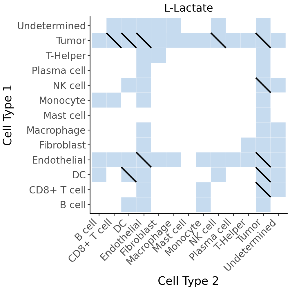
Communication heat map

To visualize the results, we will compute a communication heat map that shows the results of both hypotheses at the same time. For this, we will use the AnnData files saved previously.

gp_adata = harreman.read_h5ad('Slide_seq_lung_ct_Harreman_fix_gp.h5ad')
adata = harreman.read_h5ad('Slide_seq_lung_ct_Harreman.h5ad')

harreman.tl.select_significant_interactions(gp_adata, test = "non-parametric", ct_aware = True, threshold = 0.05)
harreman.tl.select_significant_interactions(adata, test = "non-parametric", ct_aware = True, threshold = 0.01)

cell_com_df_m_sig_gp = gp_adata.uns['ct_ccc_results']['cell_com_df_m'].copy()
cell_com_df_m_sig = adata.uns['ct_ccc_results']['cell_com_df_m'].copy()

cell_types = ['B cell', 'CD8+ T cell', 'DC', 'Endothelial', 'Fibroblast',
       'Macrophage', 'Mast cell', 'Monocyte', 'NK cell', 
       'Plasma cell', 'T-Helper', 'Tumor', 'Undetermined']

cell_com_df_m_sig_gp[['Cell Type 1', 'Cell Type 2']] = cell_com_df_m_sig_gp[['Cell Type 1', 'Cell Type 2']].replace('TAM', 'Macrophage').replace('NK', 'NK cell').replace('Misc/Undetermined', 'Undetermined')
cell_com_df_m_sig[['Cell Type 1', 'Cell Type 2']] = cell_com_df_m_sig[['Cell Type 1', 'Cell Type 2']].replace('TAM', 'Macrophage').replace('NK', 'NK cell').replace('Misc/Undetermined', 'Undetermined')

cell_com_df_m_sig_gp = cell_com_df_m_sig_gp[(cell_com_df_m_sig_gp['Cell Type 1'].isin(cell_types)) & (cell_com_df_m_sig_gp['Cell Type 2'].isin(cell_types))]
cell_com_df_m_sig = cell_com_df_m_sig[(cell_com_df_m_sig['Cell Type 1'].isin(cell_types)) & (cell_com_df_m_sig['Cell Type 2'].isin(cell_types))]

cell_com_df_m_sig_full_gp = pd.concat([
    cell_com_df_m_sig_gp,
    cell_com_df_m_sig_gp.rename(columns={'Cell Type 1': 'Cell Type 2', 'Cell Type 2': 'Cell Type 1'})
], ignore_index=True).drop_duplicates()

cell_com_df_m_sig_full = pd.concat([
    cell_com_df_m_sig,
    cell_com_df_m_sig.rename(columns={'Cell Type 1': 'Cell Type 2', 'Cell Type 2': 'Cell Type 1'})
], ignore_index=True).drop_duplicates()

cell_com_df_m_sig_full_metab_gp = cell_com_df_m_sig_full_gp[cell_com_df_m_sig_full_gp['metabolite'] == 'L-Lactate'].copy()
cell_com_df_m_sig_full_metab = cell_com_df_m_sig_full[cell_com_df_m_sig_full['metabolite'] == 'L-Lactate'].copy()

diag_lines = cell_com_df_m_sig_full_metab_gp[cell_com_df_m_sig_full_metab_gp['selected']].copy()

# For plotting diagonal lines, define tile corners
diag_lines['x'] = diag_lines['Cell Type 2']
diag_lines['y'] = diag_lines['Cell Type 1']
diag_lines['xend'] = diag_lines['Cell Type 2']
diag_lines['yend'] = diag_lines['Cell Type 1']

# Map to numeric (for line coordinates)
val_sum = 0.5
x_order = {k: i+1 for i, k in enumerate(cell_types)}
diag_lines['x0'] = diag_lines['x'].map(x_order) - val_sum
diag_lines['x1'] = diag_lines['x'].map(x_order) + val_sum
diag_lines['y0'] = diag_lines['y'].map(x_order) - val_sum
diag_lines['y1'] = diag_lines['y'].map(x_order) + val_sum

p = (
    ggplot(cell_com_df_m_sig_full_metab, aes(x='Cell Type 2', y='Cell Type 1')) +
    # Base tiles
    geom_tile(aes(fill='selected'), color='white', show_legend=False) +
    scale_fill_manual(values={True: '#C6DBEF', False: 'white'}) +

    # Diagonal lines for second condition
    geom_segment(
        diag_lines,
        aes(x='x1', y='y0', xend='x0', yend='y1'),
        color='black',
        size=1
    ) +

    # Aesthetics
    theme_classic() +
    theme(axis_text_x=element_text(rotation=45, ha='right', size=12),
            axis_text_y=element_text(size=12),
            axis_title_x=element_text(size=14),
            axis_title_y=element_text(size=14),
            figure_size=(5, 5)) +
    labs(x='Cell Type 2', y='Cell Type 1', fill='-log10(FDR)', title='L-Lactate')
)
p

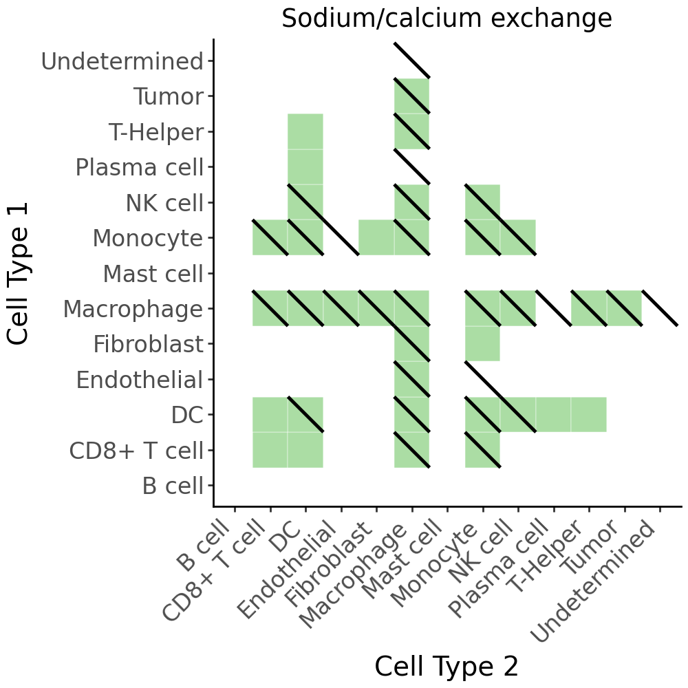
cell_com_df_m_sig_full_metab_gp = cell_com_df_m_sig_full_gp[cell_com_df_m_sig_full_gp['metabolite'] == 'Sodium_calcium exchange'].copy()
cell_com_df_m_sig_full_metab = cell_com_df_m_sig_full[cell_com_df_m_sig_full['metabolite'] == 'Sodium_calcium exchange'].copy()

diag_lines = cell_com_df_m_sig_full_metab_gp[cell_com_df_m_sig_full_metab_gp['selected']].copy()

# For plotting diagonal lines, define tile corners
diag_lines['x'] = diag_lines['Cell Type 2']
diag_lines['y'] = diag_lines['Cell Type 1']
diag_lines['xend'] = diag_lines['Cell Type 2']
diag_lines['yend'] = diag_lines['Cell Type 1']

# Map to numeric (for line coordinates)
val_sum = 0.5
x_order = {k: i+1 for i, k in enumerate(cell_types)}
diag_lines['x0'] = diag_lines['x'].map(x_order) - val_sum
diag_lines['x1'] = diag_lines['x'].map(x_order) + val_sum
diag_lines['y0'] = diag_lines['y'].map(x_order) - val_sum
diag_lines['y1'] = diag_lines['y'].map(x_order) + val_sum

p = (
    ggplot(cell_com_df_m_sig_full_metab, aes(x='Cell Type 2', y='Cell Type 1')) +
    # Base tiles
    geom_tile(aes(fill='selected'), color='white', show_legend=False) +
    scale_fill_manual(values={True: '#ABDDA4', False: 'white'}) +

    # Diagonal lines for second condition
    geom_segment(
        diag_lines,
        aes(x='x1', y='y0', xend='x0', yend='y1'),
        color='black',
        size=1
    ) +

    # Aesthetics
    theme_classic() +
    theme(axis_text_x=element_text(rotation=45, ha='right', size=12),
            axis_text_y=element_text(size=12),
            axis_title_x=element_text(size=14),
            axis_title_y=element_text(size=14),
            figure_size=(5, 5)) +
    labs(x='Cell Type 2', y='Cell Type 1', fill='-log10(FDR)', title='Sodium/calcium exchange')
)
p

Cell-type-specific interacting cell scores

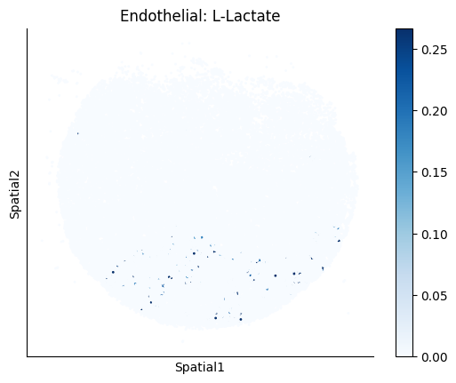
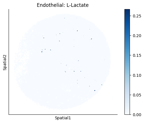
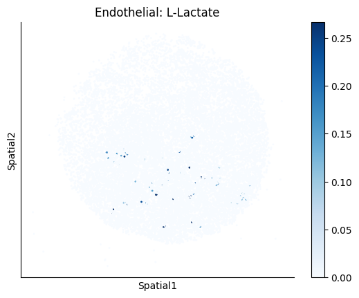
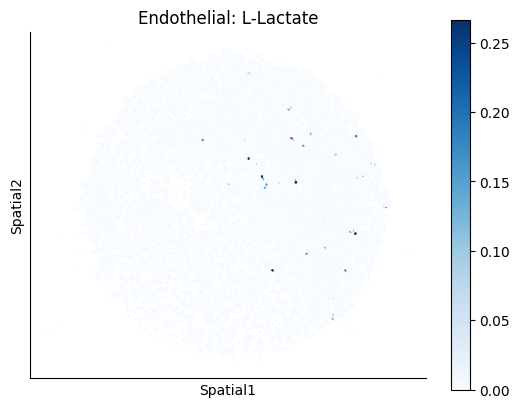
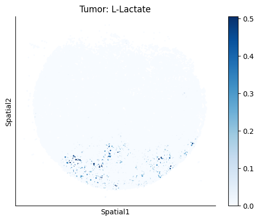
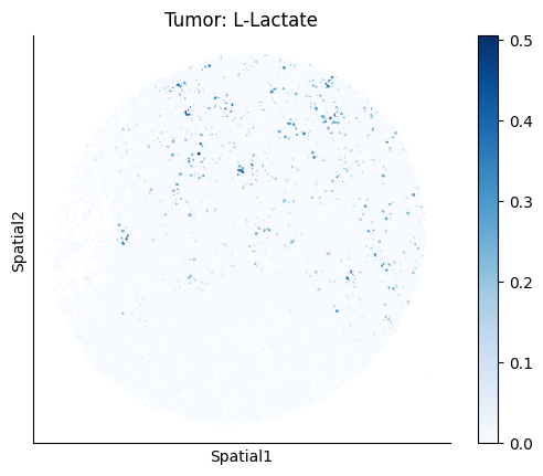
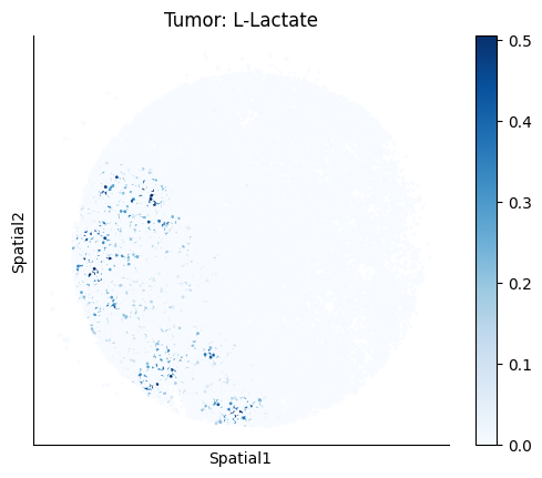
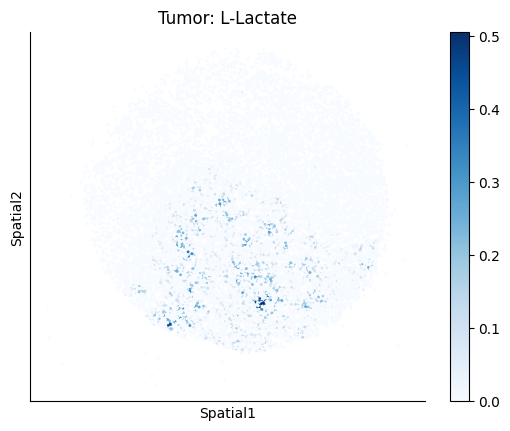
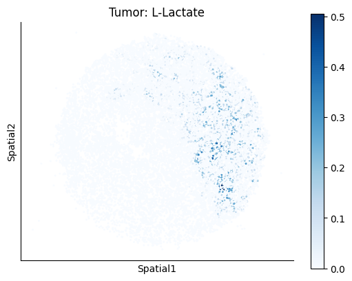
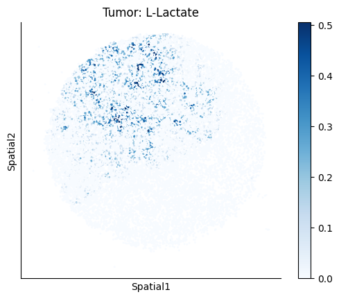
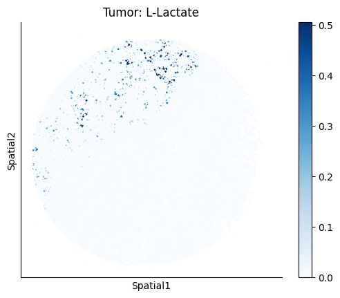
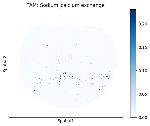
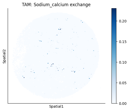
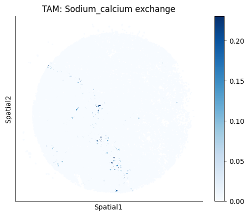
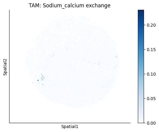
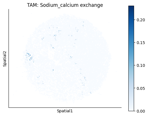
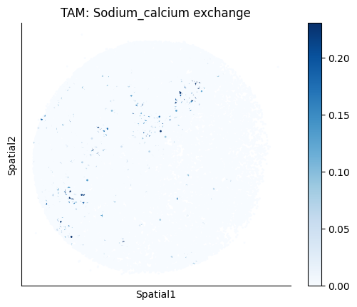
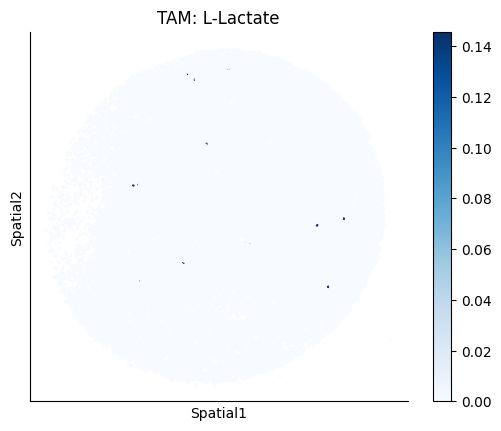
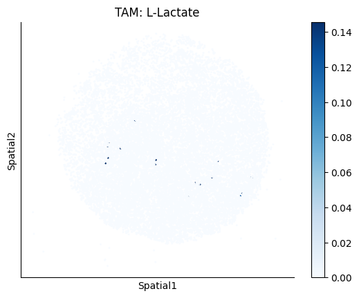
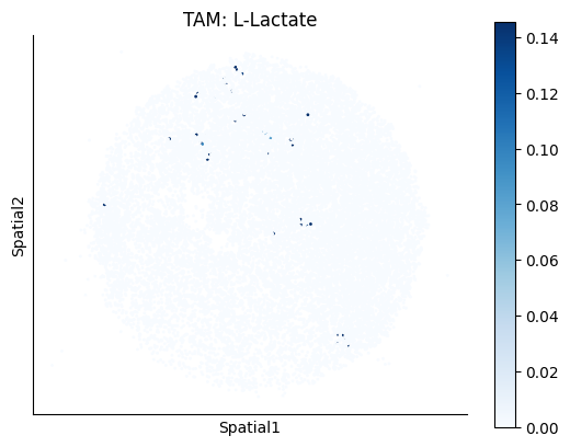
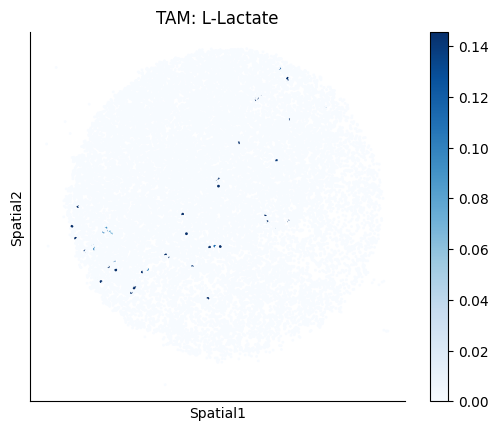
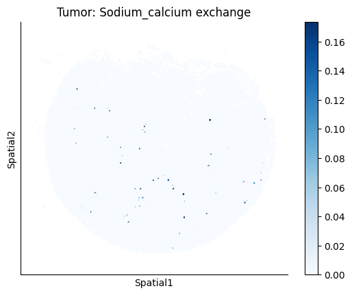
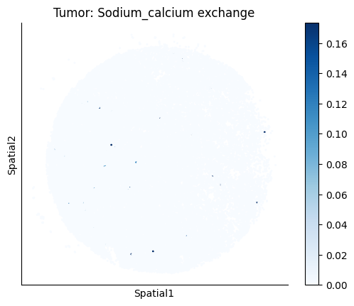
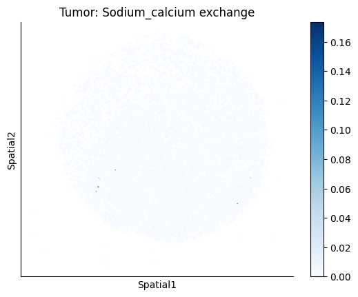
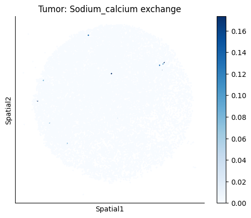
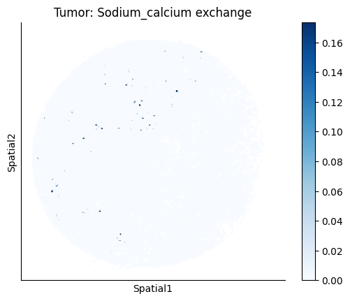
Finally, we visualize the cell-type-specific interacting cell scores with the plot_ct_interacting_cell_scores function. For this, we can select the metabolites or gene pairs of interest through the interactions parameter and the cell types of interest through the cell_type_pair parameter. The latter accepts either a list of cell types (which visualizes every pair a given cell type is part of) or a list of cell type pairs (tuples), where we only visualize the interacting scores corresponding to the specified cell type pairs. Here, we also use the agg_only = True parameter, which aggregates for the cell types of interest the interaction scores in which a given cell type is present and visualizes only these scores.

harreman.pl.plot_ct_interacting_cell_scores(adata, interactions=['L-Lactate', 'Sodium_calcium exchange'], cell_type_pair=['Tumor', 'TAM', 'Endothelial'], agg_only=True, 
                                            test='non-parametric', coords_obsm_key='spatial', s=1, vmin=0, vmax='p99.9', normalize_values=True, cmap='Blues', sample_specific=True)

Puck_220408_20
Puck_220408_13
Puck_220408_15
Puck_200727_09
Puck_200727_10
Puck_200727_08
Puck_220408_14
Puck_220408_20
Puck_220408_13
Puck_220408_15
Puck_200727_09
Puck_200727_10
Puck_200727_08
Puck_220408_14
Puck_220408_20
Puck_220408_13
Puck_220408_15
Puck_200727_09
Puck_200727_10
Puck_200727_08
Puck_220408_14
Puck_220408_20
Puck_220408_13
Puck_220408_15
Puck_200727_09
Puck_200727_10
Puck_200727_08
Puck_220408_14
Puck_220408_20
Puck_220408_13
Puck_220408_15
Puck_200727_09
Puck_200727_10
Puck_200727_08
Puck_220408_14